Texture Representation
- Contrast to object classification, the global spatial information is less important.
Bag-of-Word based methods (BoW)
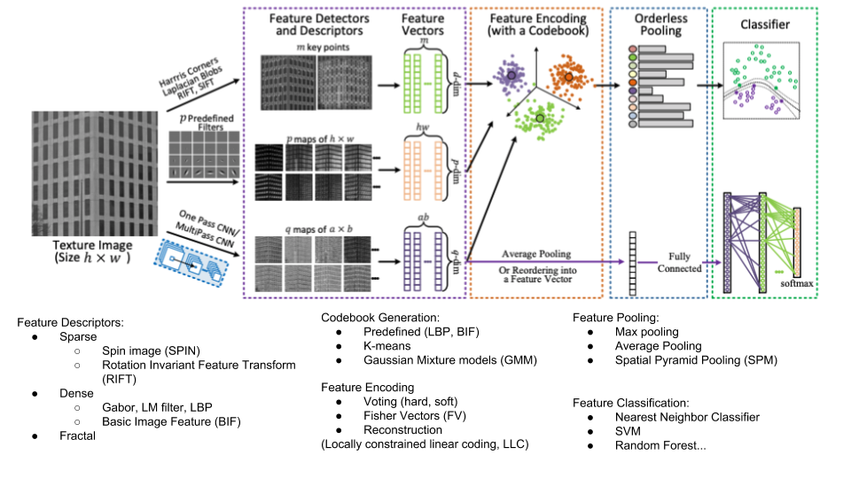
- Local Patch Extraction
- Local Patch Representation (Feature Descriptors)
- Ideal: distinctive, robust to variations
- Codebook Generation
- Find a set of prototype features from training data.
- Like words, phrases in languages. (Similar to dimension reduction)
- Feature Encoding
- Assign local representation to some prototype features.
- Feature Pooling
- Feature Classification
Convolutional Neural Network based methods
Pre-trained Generic CNN models
- CNN = convolution + non-linear activation + pooling
- Related to LBP, Random Projection (RP), etc.
- CNN-extracted features can be encoded by BoW-based method.
Fine-tuned CNN models
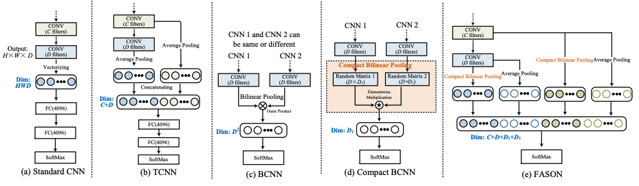
- Texture CNN (T-CNN)
- Energy Layer: average activation ouput for each feature map of the last conv layers.
- 1 value per feature map
- Similar to energy response of a filter bank.
- Example: 256x27x27 (channel x height x width) \(\rightarrow\) 256x1
- Concat: GlobalAveragePooling(intermediate conv.) and last conv.
- Insight:
- Fine-tune a texture-centric pretrained network performs better than that pretrained with object-centric dataset.
- Bilinear CNN (BCNN)
- Replace FC layers with orderless bilinear pooling layer. (Matrix outer product + aveage pooling)
- \(f(l, I)\): Feature function, l = locations, I = image
-
\[f: L \times I \rightarrow R^{K\times D}\]
- Cost: High dimenstional features \(\rightarrow\) need lots of training data
\[bilinear(l, I, f_A, f_B) = f_A(l, I)^{T}f_B(l, I)\]
\[V(j, k) = \sum{N}{i=1}a_k(x_i)(x_i(j) - c_k(j))\]
\[r_{ik} = x_i - c_k\]
\[e_k = \sum{N}{i=1}e_{ik} = \sum{N}{i=1}a_{ik}r_{ik}\]
- Soft-weight assignment (\(a_{ik}\))
- \(\beta\) is the smoothing factor
- \(\beta \rightarrow s_k\) where \(s_k\) is learnable
\[a_{ik} = \frac{exp(-\beta \|r_{ik}\|^2)}{\sum{K}{j=1}exp(-\beta \|r_{ik}\|^2)}\]
Texture-specific CNN models
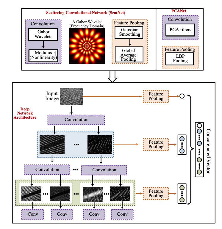
- ScatNet
- Pre-determined convolution layers (Example: Haar, Gabor wavelets)
- Translation-invariant, also extends to rotation and scale invariance.
- No need to learn, but expensive when extracting features.
- Explore theoretical aspect of CNN.
- PCANet
- Use trained PCA filters.
- Variations: RandNet, LDANet
- Faster feature extraction than ScatNet. Weaker invariance and performance.
Attribute based methods
- Allows more detail description of an image:
- Like: spotted, striated, striped, etc.
- Issues:
- Need a unified vocabulary for describing texture attribure.
- Benchmark dataset annotated by semantic attriburte.
- Studies that characterized texture attribute:
- Tamura et al.: coarseness, contrast, directionality, line-likeness, regularity and roughness
- Amadasun and King: coarseness, contrast, business, complexity, and strength (refine 1.)
- Matthews et al.: 11 commonly-used attributes by using a single adjective. (Relative comparison)
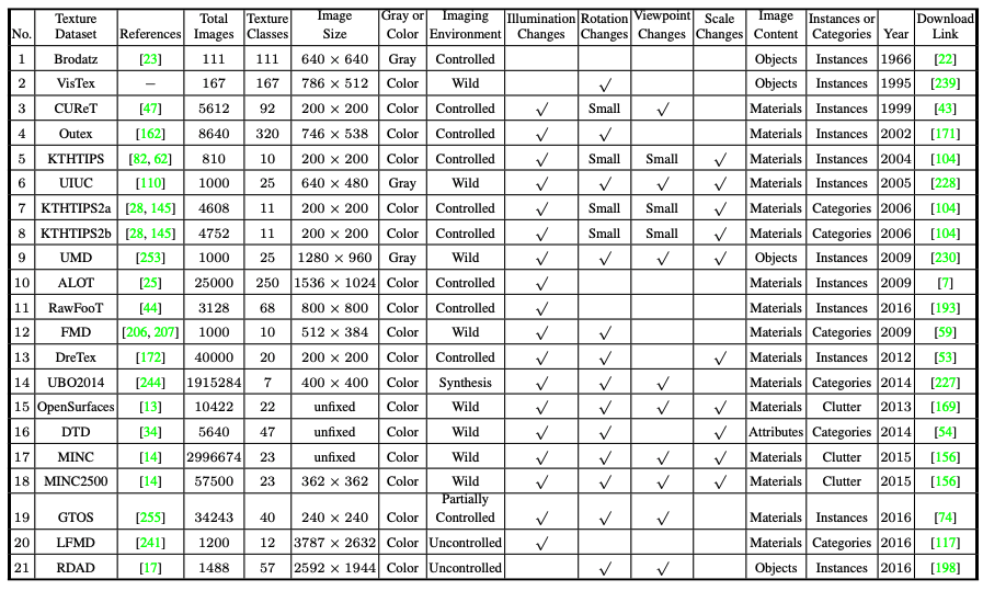
Texture Datasets