Convolutional Neural Network
This is a note of CNN model architectures.
- For what is Convolution Neural Network (CNN), I recommend you to first read this.
Image Classification
- There are pre-trained models trained on ImageNet in keras.applications.
- Pre-trained models are useful for transfer learning.
Inception (GoogLeNet)
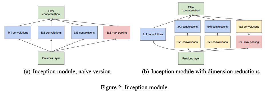
- Inception module: Various sizes of feature maps in parallel.
- Useful in localization
- Main Idea:
Finding out how an optimal local sparse structure in a convolutional vision network can be approximated and covered by readily available dense components.
- Use 1x1 convolution to reduce dimension.
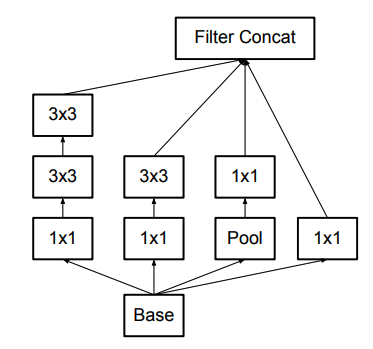
InceptionV2
| Factorized Convolution | Assymetric Convolution |
|---|---|
 |
 |
- General Design Principles:
- Avoid representational bottlenecks: avoid extreme compression to info. loss
- Increase the activation per tile in CNN: train faster
- Spatial aggregation on lower dim embed: Maybe adjacent units have strong correlation.
- Balance the width and the depth of the network.
- Factorization of convolutions:
- Replace 5x5 conv by two 3x3 convs. (Exploit translation invariance again)
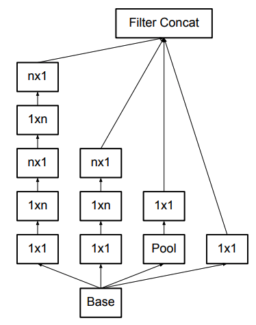
- Replace 3x3 conv by 3x1 and 1x3 convs. (nxn \(\rightarrow\) nx1 and 1xn)
- Works well on m x m feature maps (\(m = 12\sim 20\))
- Efficiently reduce grid size:
- Convolution and Pooling done seperately and concat back.
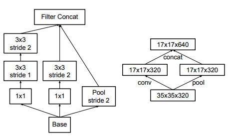
- Convolution and Pooling done seperately and concat back.
- Label-smoothing regularization (LSR): Avoid model to assign labels too confidently
- x / y = training example / label
- k = labels, u(k) = a fixed distribution (e.g. u(k) = 1/K)
- Original label distribution: \(q(k\|x) = \delta_{k,y}\)
- Smoothed label distribution: \(q'(k) = (1 - \epsilon)\delta_{k,y} + \epsilon u(k)\)
- Cross-entropy loss = \(H(q', p) = (1 - \epsilon)H(q, p) + \epsilon H(u, p)\)
- \(H(u, p)\) can be captured by KL divergence.
ResNet
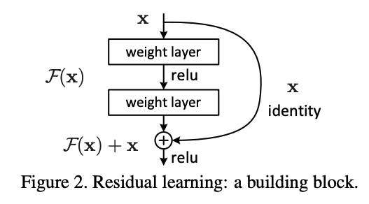
- Residual operation for reusing feature maps.
- Motivation: Deeper network produces higher training error \(\rightarrow\) Degradation.
- Core building block: (\(W_s\) is a linear projection to match dimensions) \(y = F(x, {W_i}) + W_sx\)
DenseNet
- Github
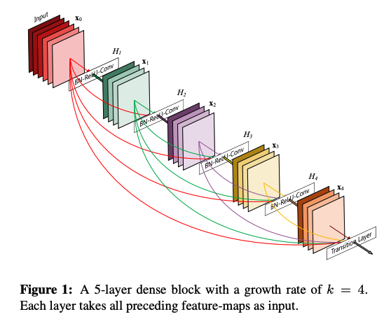
- Densely-connected convolutional layers:
- Receive concatenation of feature maps from all preceding layers.
- For \(l^{th}\) layer, the output \(x_l=H_l([x_0, x_1,..., x_{l-1}])\)
- Cannot perform pooling in Dense-connected blocks.
- Advantages:
- Universal access of feature maps within Dense blocks.
- Can reduce number of feature maps by 1x1 conv between Dense blocks.
- Deep supervision, Feature reusage, Network compression.
MobileNet
- Essence:
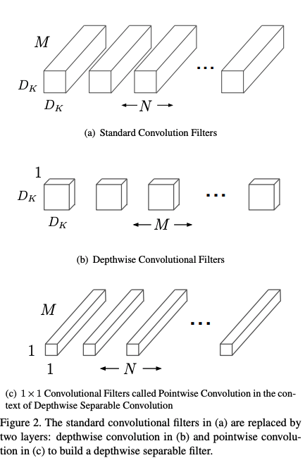
The MobileNet model is based on depthwise separable convolutions which is a form of factorized convolutions which factorize a standard convolution into a depthwise convolution and a 1×1 convolution called a pointwise convolution.
-
Seprate standard convolutional layer into 2 layers (With BatchNormalization and ReLU for layer outputs)
- Let:
- \(D_{F/G}\) = spatial dimention of feature map \(F/G\)
- \(D_K\) = spatial dimention of kernel \(K\)
- \(M\) = number of input channel, \(N\) = number of output channel
- Standard Convolution
-
Assuming stride=1 and padding \(G_{k,l,n} = \sum_{i,j,m}{K_{i,j,m,n}F_{ {k+i-1},{l+j-1},m} }\) \(i=row, j=col, m=input\space channel, n=output\space channel\)
- Parameter size of \(K = D_K\times D_K\times M\times N\)
- Computation cost = \(D_K\cdot D_K\cdot M\cdot N\cdot D_F\cdot D_F\)
-
- Depthwise separable Convolution = Depthwise & Pointwise convolution
- Depthwise convolutions: 1 filter per input channel
\(\hat{G}_{k,l,m} = \sum_{i,j}{\hat{K}_{i,j,m}F_{ {k+i-1},{l+j-1},m} }\)
- Parameter size of \(\hat{K} = D_K\times D_K\times M\)
- Computation cost = \(D_K\cdot D_K\cdot M\cdot D_F\cdot D_F\)
- Pointwise convolutions = 1x1 convolution
- Computation const = \(M\cdot N\cdot D_F\cdot D_F\)
- Further reduction of cost:
- Width parameter: \(0 < \alpha <= 1\)
- Resolution parameter: \(0 < \rho < =1\)
- Computation const = \(D_K\cdot D_K\cdot \alpha M\cdot \rho D_F\cdot \rho D_F + \alpha M\cdot \alpha N\cdot \rho D_F\cdot \rho D_F\)
- Depthwise convolutions: 1 filter per input channel
\(\hat{G}_{k,l,m} = \sum_{i,j}{\hat{K}_{i,j,m}F_{ {k+i-1},{l+j-1},m} }\)
MobileNet_v2
| Overall Architecture | Inverted Residual |
|---|---|
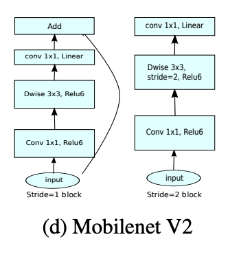 |
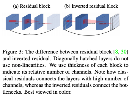 |
- Main contribution: inverted residual with linear bottleneck
- Linear bottleneck:
- Assume the “manifold of interest” lies in a low-dimensional subspace of the input space.
- Bottleneck Residual Block (\(F(x) = [A\circ N\circ B]x\)): Composition of 3 operators
- Linear transformation: \(A: R^{s\times s\times k} \rightarrow R^{s\times s\times n}\)
- Non-linear per channel: \(N: R^{s\times s\times n} \rightarrow R^{ {s}'\times {s}'\times n}\)
- In this paper: \(N = ReLU6\circ dwise\circ ReLU6\)
- Linear transformation: \(B: R^{ {s}'\times {s}'\times n} \rightarrow R^{ {s}'\times {s}'\times {k}'}\)
- Represent inner tensor \(I\) as concatenation of \(t\) tensors of size \(n/t\) \(F(x) = \sum^t_{i=1}(A_i\circ N\circ B_i)(x)\)
- Get improvement because of
- Inner transformation is per-channel.
- Consecutive non-per-channel operators have significanct \(\frac{input\space size}{output\space size}\).
- Recommended \(t = 2\sim 5\) for avoiding cache miss in matrix multiplication.
Neural Arichitecture Search (NASNet)
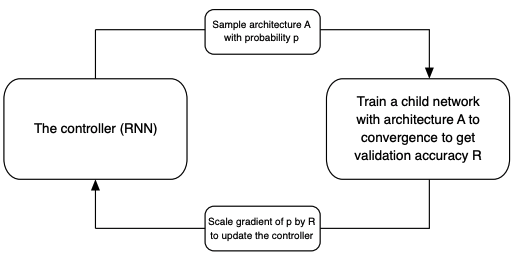
- Search architecture for building blocks on smaller dataset and transfer to larger dataset.
-
Use Reinforcement Learning to search building blocks.
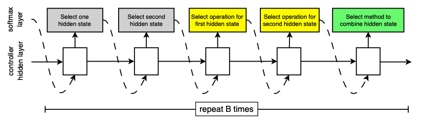
- Two main blocks (Cells):
- Normal Cell: convolutional cell that return the same dimension.
- Reduction Cell: Heigh and width is reduced by factor of 2.
- Operations: Use common operation like conv, max-pooling, depthwise-seperable conv.
- Combination of 2 hidden states:
- Element-wise addition
- Concatenation
- Controller RNN: one-layer LSTM with softmax predictions for each decision.
Object Detection & Segmentation Using CNN
- For object detection & segmentation tasks, models need to output more fine-grained details.
- Thus, many other architectures and training schema for more efficiency were proposed.
What is mAP?
Region-based CNN (R-CNN)
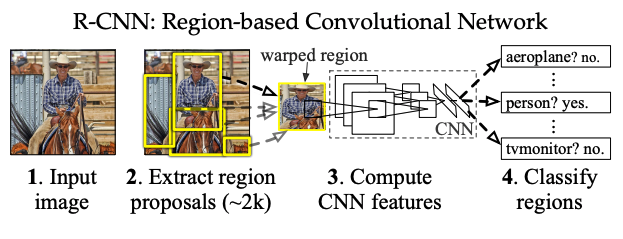
- Flow: region proposals \(\rightarrow\) CNN feature extraction \(\rightarrow\) Image classification \(\rightarrow\) BBOX regression
- Region proposals: category-independent methods
- Examples: objectness, selective search, …etc.
- CNN feature extraction: this paper use OxfordNet and TorontoNet
- Pre-trained on ILSVRC2012 (image classification labels)
- Fine-tuning on warped region proposals
- Treat all region proposals with >= 0.5 IoU as positive
- Add 1 additional background class
- Image classification: Use class-specific linear SVMs
- Grid search the overlap threshold (\(IoU = 0.1\sim 0.5\))
- Bounding Box regression:
- Linear regression with ridge regularization.
Spatial pyramid pooling networks (SPPnets):
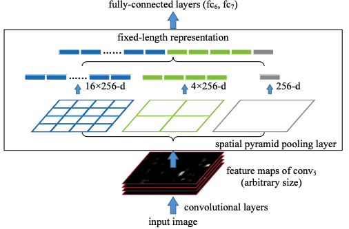
- To remove fixed size constraint in the convolution parts.
- Spatial Pyramid Pooling (SPP):
- Partition images into various size and aggregate them.
- SPPnet:
- Replace the last pooling layer with SPP layer.
- SPP layer outputs: \(kM\)-dimensional vectors
- \(M\) = the number of spatial bins
- \(k\) = the number of filters in the last convolutional layer
Fast R-CNN
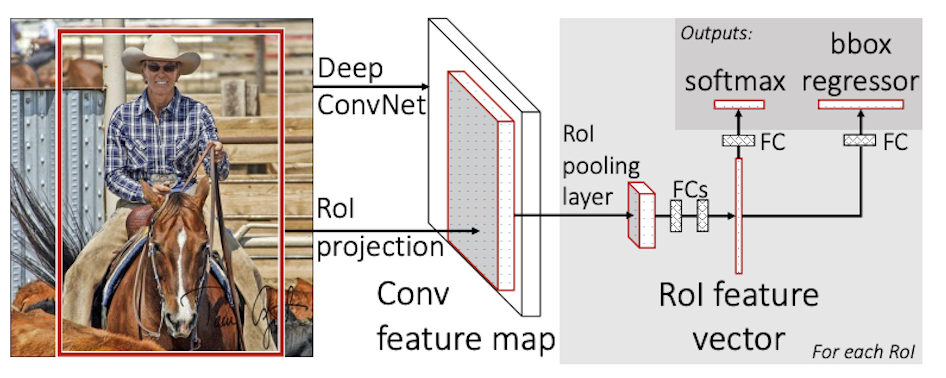
- RoI pooling layer: Only one pyramind level in SPPnets
- Initialization: pre-trained ImageNet network with 3 modification
- Replaced last max-pooling by RoI pooling layer.
- Add a FC and softmax over K + 1 classes and bbox regressors.
- Modify input into: a list of images and RoIs for each images.
- Comparison with R-CNN and SPPnet:
- Fast R-CNN: For each batch, use RoIs from small set of images.
- End-to-End training for fine-tuning, classification, bbox regression.
- Multi-task loss:
- \([u\geq 1]\) = 1 if \(u\geq 1\) else 0 (background class: u = 0)
- \(L_{cls}(p,u) = -logp_u\) is the log loss for true class \(u\)
-
\[L_{loc}(t^u,v) = \sum_{i\in {x,y,w,h} } smooth_{L_1}(t^u-v_i)\]
- \(L_1\) loss: less sensitive to outliers and prevent exploding gradient.
- Speed up for detection using Truncated SVD
- Motivation: Slow when many RoI vectors forward-pass fully-connected layers (\(W\)).
- Factorize \(W\) as \(W \approx U\sum_t V^T\) (\(U: u\times t\), \(\sum_t: t\times t\), \(V^T: v\times t\))
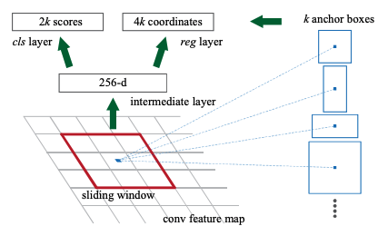
Faster R-CNN (Region Proposal Network(RPN))
- Motivation: Region proposals cause computation bottleneck
- Faster R-CNN = RPN + Fast R-CNN
- RPN: 2 additional conv layers (a kind of FCN)
- Encodes each position in feature map into a fixed-length vector. (nxn conv.)
- Score each vector an objectness score and regressed bbox for \(k\) region proposals of various scale. (1x1 conv.)
- Translation-Invariant Anchors: a set of pre-defined bboxes
- Each anchor can have different scales and aspect ratios
- Here they use 3 scales and 3 aspect ratios, resulting in 9 anchors at each position
- Each anchor can have different scales and aspect ratios
- Loss function for learning region proposals
- Labels for each anchor (object or background):
- Positive:
- Highest IoU with ground-truth bboxes.
- IoU with ground truth \(\geq\) threshold (e.g. 0.7)
- Negative: IoU \(\leq\) threhold (e.g. 0.3) with all ground-truth bboxes.
- Positive:
- Multi-task loss: \(L({p_i},{t_i}) = \frac{1}{N_cls} \sum_i L_{cls}(p_i,p_i^*) + \lambda \frac{1}{N_reg} \sum_i p_i^*L_{reg}(t_i,t_i^*)\)
- \(p_i\) = predicted probability of anchor \(i\) being an object. (\(p_i^*\) = true label)
- \(t_i\) = a vector of bbox coordinates. (\(t_i^*\) = true coordinates)
- \(L_{cls}(p_i,p_i^*)\) = log loss over 2 classes
- \(L_{reg}(t_i,t_i^*)\) = smoothed L1-loss in Fast-RCNN
- Labels for each anchor (object or background):
- Share conv features between RPN and Fast R-CNN: 4-step training
- Train RPN (with ImageNet-pre-trained model and fine-tune end-to-end)
- Train Fast R-CNN using proposals from 1.
- Initialze RPN and fine-tune RPN with fixed shared conv layers.
- Fine-tune Fast R-CNN with fixed shared conv layers.
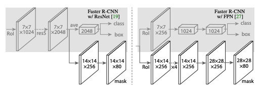
Mask R-CNN
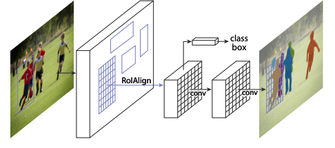
-
Add mask branch (FCN) for image segmentation into Faster R-CNN.
- Multi-task loss for each RoI: \(L = L_{cls} + L_{box} + L_{mask}\)
- \(L_{cls},L_{box}\) are the same as Faster R-CNN
- \(L_{mask}\) is the average binary cross-entropy loss of pixel-wise masks.
- \(K\) binary masks of resolution \(m x m\) for \(K\) classes.
- Decouple classification and segmentation by per-pixel sigmoid and binary loss.
- To fix misalignment, a quantization-free layer: RoIAlign
- Use bilinear interpolation to compute exact values of input feature.
- No quantization is the most crucial point.
- Network:
Feature Pyramid Networks (FPN)
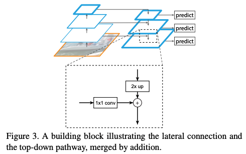
- Main Goal:
The goal of this paper is to naturally leverage the pyramidal shape of a ConvNet’s feature hierarchy while creating a feature pyramid that has strong semantics at all scales.
- To construct multi-scale feature maps for downstream tasks.
- Utilize each level of conv-layers to produce multi-scale feature maps.
- Each level of feature maps = Upsampling(Higher level) + Conv1x1(Current level)
- Applications:
- For Region-proposal Network (RPN):
- Attach the RPN head (3x3 conv and 2 1x1 convs) to each level of feature pyramid.
- Each anchor has single scale, multiple aspect ratios for each level.
- For Fast R-CNN:
- Assign an RoI of width \(w\) and height \(h\) to level \(P_k\) by: \(k = \lfloor{k_0 + log_2(\sqrt{wh}/224)}\rfloor\)
- \(k_0\) = target level that RoI mapped into
- 224 is the canonical ImageNet pre-training size
- Attach predictor heads to all RoIs of all levels.
- Assign an RoI of width \(w\) and height \(h\) to level \(P_k\) by: \(k = \lfloor{k_0 + log_2(\sqrt{wh}/224)}\rfloor\)
- For Region-proposal Network (RPN):
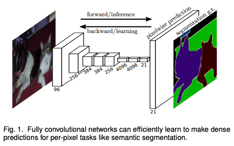
Fully Connected CNN (FCN)