Pandas
![]()
在蟒蛇的眼裡,熊貓是很會分析資料的!
- Pandas是以numpy為基礎,加上許多處理表格資料的功能的一個package。
- Full documentation: https://pandas.pydata.org/pandas-docs/stable/
- 更詳細的資料結構教學:https://pandas.pydata.org/pandas-docs/stable/getting_started/dsintro.html?highlight=dataset
pip3 install pandas
- 主要就是分成1D和2D的表格資料結構:
- Series
- DataFrame
In [75]:
import pandas as pd
import numpy as np
from os.path import join
讀取檔案:
- sep: 指定分開數值的標點符號:常用有','、'\t'、' '。
- index_col: 指定當作index的欄位(=0表示指定第一個column)
header: 指定哪一行當作column名稱(=0表示指定第一行)
DataFrame.head(n): 顯示前n筆資料
In [54]:
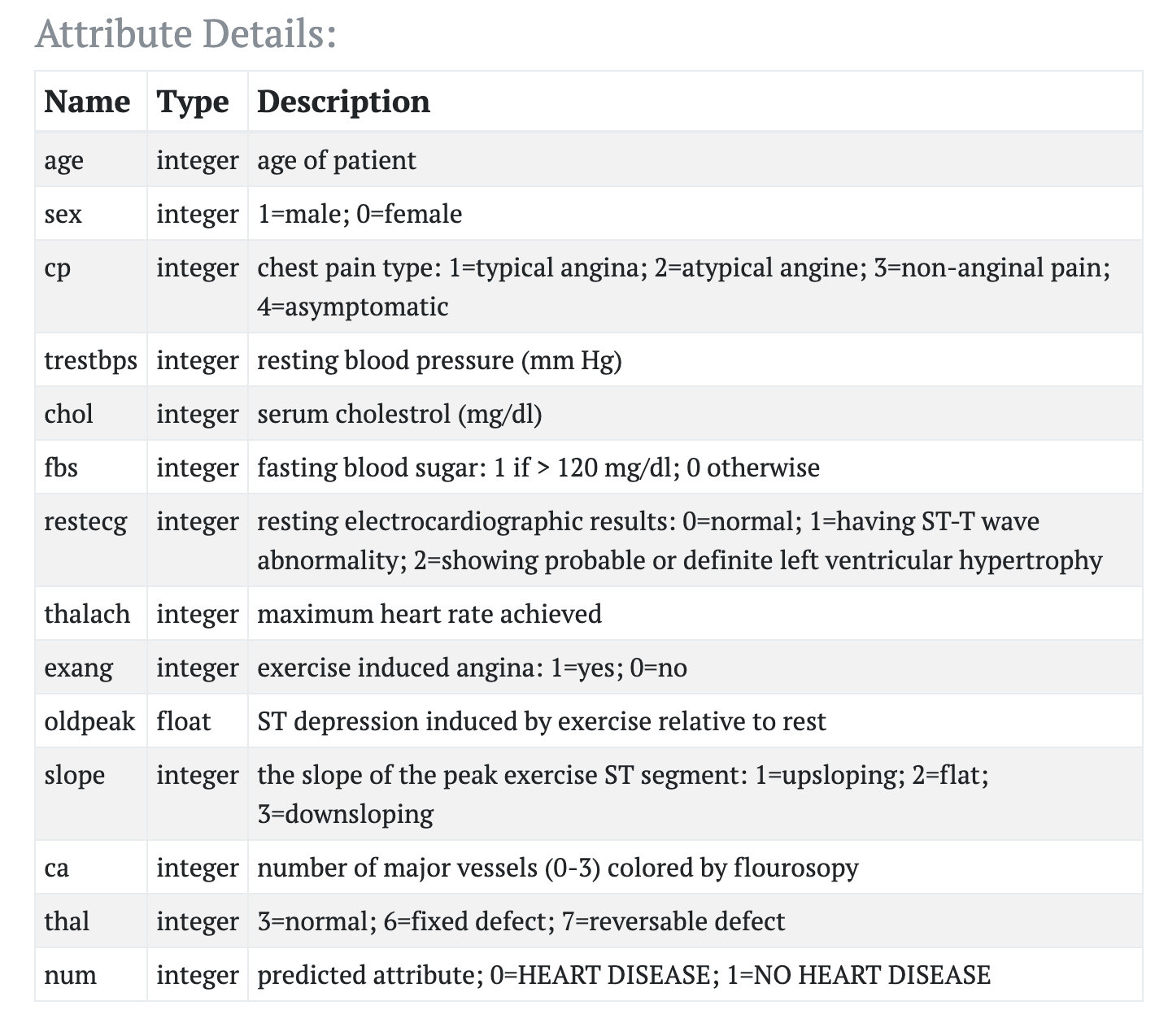
data = pd.read_csv(join("data", "heart_disease_dataset.csv"), sep=',',
                  index_col=None, header=0)
data.head(3)
Out[54]:
In [55]:
print(type(data), data.shape)
In [56]:
data.describe()
Out[56]:
選取資料:
- 如果只選擇一個row/column,選到的東西就是一個Series。
.iloc[]: 用數字index選取.loc[]: 用名稱選取- 用條件選取
In [57]:
age = data.loc[:, 'age']
patient0 = data.iloc[0, :]

chestpain_and_sex = data.loc[:, ['cp', 'sex']]
print(type(patient0), type(age), type(chestpain_and_sex))
In [58]:
female = data[data.sex == 0]
female.shape
Out[58]:
更改資料:
- 換row/column名字:
- 直接改
.index和.columns - 自動編號:
reset_index(), set_index()
- 直接改
- 更改數值:
- NA:
fillna(VAL), dropna(): 當表格中有缺失值時,可以一步填補或丟棄。 - apply:
.apply(FUN, axis, ...): 將每個row(axis=1)/column(axis=0)送進FUN處理並回傳,簡潔又比for-loop還快速。
- NA:
In [59]:
data.index = ['patient{}'.format(i) for i in data.index]
data.columns = data.columns[:-1].tolist() + ['predict_target']
data.head(5)
Out[59]:
In [60]:
reset_data = data.reset_index()
reset_data.head(2)
Out[60]:
In [61]:
age_index_data = data.set_index(['age'])
age_index_data.head(2)
Out[61]:
In [62]:
gender = {1: "male", 0: "female"}

gender_data = data.apply(lambda x: gender[x.sex], axis=1)
gender_data1 = data['sex'].apply(lambda x: gender[x])
(gender_data == gender_data1).all()
Out[62]:
In [63]:
%%timeit
gender_data = data.apply(lambda x: gender[x.sex], axis=1)
In [64]:
%%timeit
gender_data = []
# .iterrows() 可以一行一行進入for-loop,每一行會分成(index, 該row的series)
for index, series in data.iterrows():
    gender_data += [gender[series.sex]]

gender_data = pd.Series(gender_data, index=data.index)
分類資料: groupby
- 按照指定column的內容分成數群,並對每一群作相同或不同的操作。
- 通常分群之後,我們可能會想對資料做下面任何一種動作:
- Aggregation: 計算一些摘要的統計值。
- Transformation: 對資料做一些轉換,例如對每一群各自標準化。
- Filtration: 對每一組以不同條件過濾資料。
In [67]:
data.groupby('predict_target').mean()
Out[67]:
In [73]:
for group_name, group in data.groupby('cp'):

    chest_pain_group = group.groupby('predict_target').count()
    no_d = chest_pain_group.iloc[0,0]
    is_d = chest_pain_group.iloc[1,0]

    print("Group name {}: No disease: {}, Heart disease: {}".format(group_name, no_d, is_d))
In [78]:
# 對每一組的剩下column都計算mean, std和count。
data.groupby('cp').agg([np.mean, np.std, 'count'])
Out[78]:
合併資料
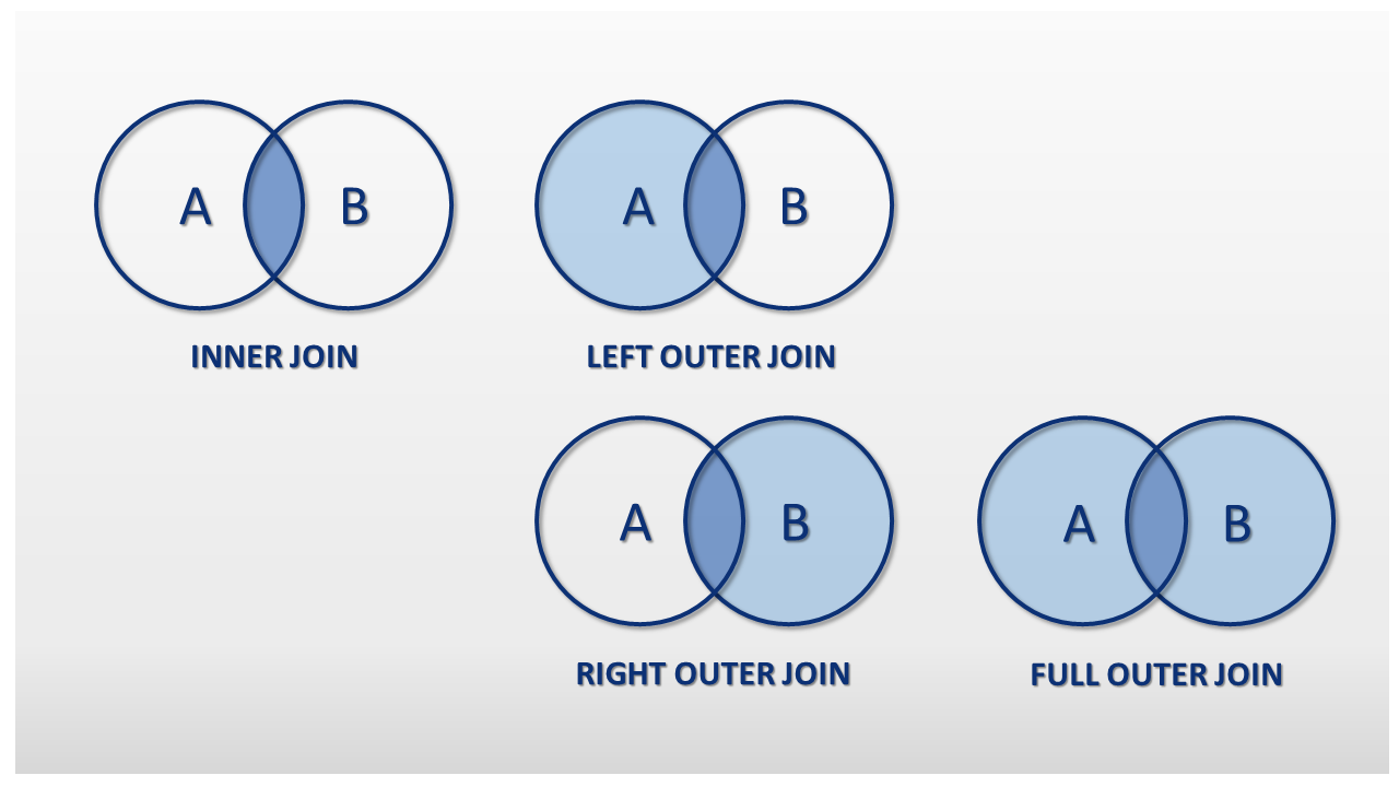
concat: 將別的DataFrame和原本的接在ㄧ起,可以接在新的rows或是columns,但是dimension要一樣。append: 將新的row接在原本的DataFrame下面。join: 將另一個DataFrame的column接到原本的右邊。
merge: 跟SQL很像的合併資料方式,可以合併相同的column。- 合併資料的方式大致可以分成"left join", "right join", "inner join", "outer join"
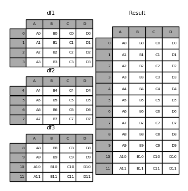
In [81]:
df1 = pd.DataFrame({'A': ['A0', 'A1', 'A2', 'A3'],
                     'B': ['B0', 'B1', 'B2', 'B3'],
                     'C': ['C0', 'C1', 'C2', 'C3'],
                     'D': ['D0', 'D1', 'D2', 'D3']},
                    index=[0, 1, 2, 3])


df2 = pd.DataFrame({'A': ['A4', 'A5', 'A6', 'A7'],
                     'B': ['B4', 'B5', 'B6', 'B7'],
                     'C': ['C4', 'C5', 'C6', 'C7'],
                     'D': ['D4', 'D5', 'D6', 'D7']},
                    index=[4, 5, 6, 7])


df3 = pd.DataFrame({'A': ['A8', 'A9', 'A10', 'A11'],
                     'B': ['B8', 'B9', 'B10', 'B11'],
                     'C': ['C8', 'C9', 'C10', 'C11'],
                     'D': ['D8', 'D9', 'D10', 'D11']},
                    index=[8, 9, 10, 11])

result = pd.concat([df1, df2, df3])
- concat之前和之後的結果
In [ ]:
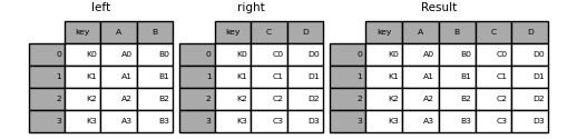
left = pd.DataFrame({'key': ['K0', 'K1', 'K2', 'K3'],
                     'A': ['A0', 'A1', 'A2', 'A3'],
                     'B': ['B0', 'B1', 'B2', 'B3']})


right = pd.DataFrame({'key': ['K0', 'K1', 'K2', 'K3'],
                      'C': ['C0', 'C1', 'C2', 'C3'],
                      'D': ['D0', 'D1', 'D2', 'D3']})


result = pd.merge(left, right, on='key')
Practice:
- 將'data/wpbc.data'的每個column按照'data/wpbc.names'的說明取名字。
In [166]:
df = pd.read_csv(join('data', 'wpbc.data'), sep=',')
In [79]:
import matplotlib.pyplot as plt
import seaborn as sns
In [104]:
t = np.arange(0., 5., 0.2)

# red dashes, blue squares and green triangles
plt.plot(t, t, 'r--', t, t**2, 'bs', t, t**3, 'g^', t, t**(0.5), 'y.')
plt.show()
plt.close()

Seaborn
- 基於Matplotlib所寫的視覺化package,用更high-level的函數畫出更好看的圖表^ ^
- 如果用pandas的資料型態,seaborn會直接用row/column的名字當作圖的label。
Full documentation: https://seaborn.pydata.org/index.html
基本上用來視覺化的資料可以有四種:
- Vectors of data: 用lists、numpy arrays或是pandas Series表示的資料。
- Long-form DataFrame (stacked data): 一個column記錄數值、其他column記錄該數值的意義。
- Wide-form DataFrame (unstacked data): 每個column都代表不同的資料特性,會各自被當成x軸的一類,
- An array or a list of 1.
In [124]:
plt.style.use('seaborn-dark')

tips = sns.load_dataset("tips")
tips.head(3) # wide-form
Out[124]:
In [128]:
groups = tips.groupby(["sex", "day"]).mean().total_bill
In [163]:
sns.set_context("talk") # "poster", "paper"
fig, ax = plt.subplots(2, 2, figsize=(15,12))

sns.barplot(x='sex', y='total_bill', data=tips, ax=ax[0][0])

sns.scatterplot(x='tip', y='total_bill', data=tips, ax=ax[0][1],
               hue='size', palette='Set2', style='smoker')

sns.boxplot(x='time', y='tip', data=tips, ax=ax[1][0])

sns.heatmap(groups.unstack(), ax=ax[1][1], annot=True, fmt=".1f",
            cmap='coolwarm')

ax[1][1].set_title("Average total bill")


plt.tight_layout() # 讓圖表們可以盡量不重疊又節省空間
plt.show()
plt.close()


More plotting style
In [ ]:
print(plt.style.available)
plt.style.use('fivethirtyeight')
Practice:
- 選擇seaborn裡面其中一個dataset,用至少四種圖表視覺化資料中的任意關係。
- 將圖檔以dpi=600的解析度存下來。
In [159]:
print(sns.get_dataset_names())
Out[159]:
- 其實pandas也可以.....